Chapter 4 (English)
| Site: | AssessmentKaro |
| Course: | Operating Systems |
| Book: | Chapter 4 (English) |
| Printed by: | Guest user |
| Date: | Saturday, 18 July 2026, 4:52 PM |
Description
 Topic wise chapter (English)
1. Mass Storage Structure
Mass Storage Structure – Overview in OS
Mass storage refers to non-volatile storage devices used by an operating system to store data permanently. This includes hard disk drives (HDDs), solid-state drives (SSDs), optical disks, and other large-capacity storage media. The OS manages these devices to provide efficient, reliable access to data. The mass storage structure in OS can be understood in layers:
1. Physical Storage Layer
- Definition: The actual hardware where data is stored.
- Examples: HDD platters, SSD flash cells, magnetic tapes.
- Characteristics:
- Data is organized in blocks or sectors.
- Access times vary depending on device type.
- Storage is divided into tracks and sectors in HDDs.
2. Logical Storage Layer
- Definition: How the OS abstracts physical storage into logical units for easier management.
- Components:
- Blocks or Sectors: Smallest unit of data transfer (usually 512 bytes or 4 KB).
- Logical Block Addressing (LBA): The OS refers to storage locations using logical addresses instead of physical locations.
- Partitions: Dividing the storage device into independent logical areas, each possibly containing a file system.
3. File System Layer
- Definition: A structured way to store, retrieve, and organize files on mass storage.
- Key Functions:
- Mapping file names to data blocks.
- Managing free space and allocation.
- Maintaining metadata like file size, creation date, permissions.
- Common File Systems:
- Windows: NTFS, FAT32
- Linux: ext4, XFS
- macOS: APFS
4. Access Methods
- Definition: How the OS allows programs to read/write data.
- Types:
- Sequential Access: Data is read/written in order (e.g., tape storage).
- Direct Access (Random Access): Data can be read/written at any location (e.g., HDD, SSD).
5. Storage Management by OS
- Disk Scheduling: Optimizes read/write operations for speed (e.g., FCFS, SSTF, SCAN algorithms).
- Buffering: Temporary storage of data to balance speed differences between CPU and disk.
- Caching: Keeps frequently accessed data in faster memory (RAM).
- RAID Management: Some OSs handle Redundant Array of Independent Disks for fault tolerance and performance.
2. Disk structure
Disk Management in Operating System
Disk management is a critical function of the operating system (OS) that deals with organizing, optimizing, and securing data on secondary storage devices such as hard disk drives (HDDs) and solid-state drives (SSDs).
It ensures:
- Efficient use of storage space
- Safe and reliable read/write operations
- Faster access times
OS Management Functions
Modern operating systems implement four major management functions, and disk management is one of them:
- Process Management: handles process execution.
- Memory Management: manages main memory allocation.
- File & Disk Management: organizes data on secondary storage.
- I/O System Management: manages device communication.

Why Disk Management is Important
Most computer systems use secondary storage devices (like hard disks, SSDs, tapes, optical media, and flash drives) to store programs and data at low cost and with non-volatile storage. Data is stored in the form of files.
The operating system (OS) manages file storage by allocating disk space as needed. Files are not always stored in one continuous block, large files may be fragmented into parts stored in different disk locations, especially when space is limited.
The OS keeps track of where each file (and its fragments) is located, often handling thousands of such entries. It ensures:
- Files can be quickly located for read/write operations
- Safe and reliable access to stored data
- Efficient management of access times
Key Operations in Disk Management
Disk Formatting
- Low-level (physical) formatting: Divides the disk into sectors with headers, data, and error correction codes (ECC).
- Logical formatting: Creates a file system, defining free space and allocated space.
- Blocks are grouped into clusters for efficient I/O.
- Some systems allow raw I/O (direct access to disk blocks without a file system).
2. Booting from Disk
- The bootstrap program loads the OS kernel into memory when the computer is powered on.
- A small bootstrap loader resides in ROM.
- The full bootstrap code is stored in the boot block of the disk.
- A disk with a boot partition is called a boot disk (system disk).
3. Bad Block Management
Disks often have bad sectors due to manufacturing defects or usage.
Handled using:
- Sector sparing (replacement): faulty sectors are replaced with spare ones.
- Error recovery: for soft errors.
- Manual intervention: required for hard errors.
Severe disk failures may require replacing the disk and restoring from backup.
Some common disk management techniques used in operating systems include:
- Partitioning: Divides a physical disk into multiple logical partitions, each acting as a separate storage device for better organization.
- Formatting: Prepares a disk by creating a file system; erases all existing data.
- File System Management: Manages file systems (e.g., FAT, NTFS, ext4) to store and access data efficiently.
- Disk Space Allocation: Allocates space for files using methods like contiguous, linked, or indexed allocation.
- Disk Defragmentation: Rearranges scattered data blocks to improve performance.
3. Disk attachment
Disk Attachment
The disk attachment is a special feature that allows you to attach a disk (such as a USB flash drive) to your computer’s hard drive. Users can use this feature to store files in the cloud or transfer files between computers on their network.
Host-Attached Storage
Host-attached storage (HAS) is a form of internal computer storage that can be attached to a host computer, such as a PC or server. Host-attached devices are often used for backup purposes and can include tape drives, optical drives, hard disk drives (HDDs), solid state drives (SSDs), USB flash drives, and other similar media.
A common example of host-attached storage is the use of an external USB flash drive for data transfer between computers. This type of connection allows users to copy files from one device onto another without having to connect them directly through their operating system's file-sharing functionality - this means that you don't have access rights over your own system if someone else has access!
Host-attached storage is usually very fast, which makes it a popular choice for high-performance applications. It's also relatively cheap compared to network-attached storage (NAS), which is another form of internal computer storage that can be accessed by multiple systems at once.
Host-attached storage systems are often used in data centers because of their high performance and reliability. These devices are usually more expensive than NAS devices, but they offer many benefits over other types of internal computer storage.
Network-Attached Storage (NAS)
A Network-Attached Storage (NAS) is a computer that is connected to a network and shared by multiple users. NAS can also be called a file server, or storage appliance. The term "storage" refers to any device that stores data; this includes hard drives and flashes memory modules.
NAS has its own processor and memory so it can perform many tasks simultaneously without slowing down other devices on the network; this makes it an ideal solution for businesses who need high availability but don’t have enough CPU power available at their desktops or laptops. NAS systems are often used as backup solutions for PCs because they allow users to access files from anywhere in the world through remote access services provided by vendors such as Symantec Remote Access Server (RAS).

The NAS device is typically installed in the business’ server room and shared across the network. It can be configured for both file sharing and print serving, depending on what type of business you run. A NAS system will allow multiple users to access files simultaneously without slowing down network performance; this makes it an ideal solution for businesses that need high availability but don’t have enough CPU power available at their desktops or laptops.
Storage Area Network (SAN)
Storage area networks (SAN) are a network of storage devices that can be used to store and retrieve data from a shared central repository. A SAN is usually used for large data storage and retrieval, which requires high availability, scalability, reliability, and performance. The most common type of SAN uses fiber channel adapters to connect the host with its disk arrays.
A block-based storage protocol like Fibre Channel Protocol (FCP) allows multiple devices within the same fabric to communicate with each other in order to share resources such as disks or tape drives. In contrast to other protocols such as iSCSI or Network File System (NFS), FCP does not require any special software drivers on either end because all communication takes place using standard protocols like TCP/IP.
Another common type of SAN uses a network called InfiniBand (IB), which is a high-speed serial interconnect that provides better performance than traditional Ethernet networks. When used in conjunction with FCP, IB allows data to be transferred faster and more efficiently between two computers.
A SAN can be implemented in two ways: as an external or internal device. An external SAN is used to connect storage devices to a network, while an internal SAN is integrated into the operating system of a computer. A disk is basically a device that communicates with the host to fetch data or store data in it with the help of I/O devices.

A disk is a physical device that stores data permanently. The disk is a hardware component that is used to store data permanently.
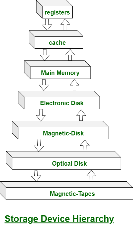
Hierarchical organization of data on disk:
- Sectors are divided into tracks and blocks within each track, each block contains sectors that are aligned on consecutive addresses;
- Tracks are divided into cylinders and heads; cylinder contains heads; heads contain sectors; sectors in every track start at address 0 (zero).
The physical organization of data on disks can be described as follows:
-A disk has multiple concentric tracks. Each track is divided into many sectors. A sector is the smallest unit of storage on a disk – it can hold one or more bytes of data (or nothing at all). Each sector is identified by its starting and ending address on the disk. The range of addresses used by a particular drive is called a cylinder head sector (CHS) addressing scheme.
-In order to find the starting address of a sector, you need to know two things: the cylinder number and head number (or track position). For example, if a disk has 100 cylinders and 40 heads, then each head can read or write data on up to 8 tracks at once.
4. Disk scheduling algorithms
Disk Scheduling Algorithms
Disk scheduling algorithms manage how data is read from and written to a computer's hard disk. These algorithms help determine the order in which disk read and write requests are processed.
- Disk scheduling is also known as I/O Scheduling.
- The main goals of disk scheduling are to optimize the performance of disk operations, reduce the time it takes to access data and improve overall system efficiency.
- Common disk scheduling methods include First-Come, First-Served (FCFS), Shortest Seek Time First (SSTF), SCAN, C-SCAN, LOOK, and C-LOOK.
Importance of Disk Scheduling in Operating System
- Multiple I/O requests may arrive by different processes and only one I/O request can be served at a time by the disk controller. Thus other I/O requests need to wait in the waiting queue and need to be scheduled.
- Two or more requests may be far from each other so this can result in greater disk arm movement.
- Hard drives are one of the slowest parts of the computer system and thus need to be accessed in an efficient manner.
Key Terms Associated with Disk Scheduling
- Seek Time: Time taken to move the disk arm to the track where data is located.
- Rotational Latency: Time taken for the desired sector to rotate under the read/write head.
- Transfer Time: Time taken to actually read or write the data, depending on disk speed and data size.
Disk Access Time = Seek Time + Rotational Latency + Transfer Time
Total Seek Time = Total head Movement * Seek Time

Disk Response Time
- Response Time: The time a request waits before its I/O operation starts.
- Average Response Time: The mean waiting time of all requests.
- Variance in Response Time: How much individual waiting times differ from the average.
Goals of Disk Scheduling Algorithms
- Minimize Seek Time
- Maximize Throughput
- Minimize Latency
- Ensuring Fairness
- Efficiency in Resource Utilization
Disk Scheduling Algorithms
There are several Disk Several Algorithms. We will discuss in detail each one of them.
- FCFS (First Come First Serve)
- SSTF (Shortest Seek Time First)
- SCAN
- C-SCAN
- LOOK
- C-LOOK
- RSS (Random Scheduling)
- LIFO (Last-In First-Out)
- N-STEP SCAN
- F-SCAN
1. FCFS (First Come First Serve)
FCFS is the simplest of all Disk Scheduling Algorithms. In FCFS, the requests are addressed in the order they arrive in the disk queue. Let us understand this with the help of an example.

Suppose the order of request is- (82,170,43,140,24,16,190) and current position of Read/Write head is: 50
So, total overhead movement (total distance covered by the disk arm) =
(82-50)+(170-82)+(170-43)+(140-43)+(140-24)+(24-16)+(190-16) =642
Advantages of FCFS
Here are some of the advantages of First Come First Serve.
- Every request gets a fair chance
- No indefinite postponement
Disadvantages of FCFS
Here are some of the disadvantages of First Come First Serve.
- Does not try to optimize seek time
- May not provide the best possible service
2. SSTF (Shortest Seek Time First)
In SSTF (Shortest Seek Time First), requests having the shortest seek time are executed first. So, the seek time of every request is calculated in advance in the queue and then they are scheduled according to their calculated seek time. As a result, the request near the disk arm will get executed first. SSTF is certainly an improvement over FCFS as it decreases the average response time and increases the throughput of the system. Let us understand this with the help of an example.
Example:

Suppose the order of request is- (82,170,43,140,24,16,190) and current position of Read/Write head is: 50
total overhead movement (total distance covered by the disk arm) =
(50-43)+(43-24)+(24-16)+(82-16)+(140-82)+(170-140)+(190-170) =208
Advantages of Shortest Seek Time First
Here are some of the advantages of Shortest Seek Time First.
- The average Response Time decreases
- Throughput increases
Disadvantages of Shortest Seek Time First
Here are some of the disadvantages of Shortest Seek Time First.
- Overhead to calculate seek time in advance
- Can cause Starvation for a request if it has a higher seek time as compared to incoming requests
- The high variance of response time as SSTF favors only some requests
3. SCAN
In the SCAN algorithm the disk arm moves in a particular direction and services the requests coming in its path and after reaching the end of the disk, it reverses its direction and again services the request arriving in its path. So, this algorithm works as an elevator and is hence also known as an elevator algorithm. As a result, the requests at the midrange are serviced more and those arriving behind the disk arm will have to wait.
Example:

Suppose the requests to be addressed are-82,170,43,140,24,16,190 and the Read/Write arm is at 50, and it is also given that the disk arm should move "towards the larger value".
Therefore, the total overhead movement (total distance covered by the disk arm) is calculated as
= (199-50) + (199-16) = 332
Advantages of SCAN Algorithm
Here are some of the advantages of the SCAN Algorithm.
- High throughput
- Low variance of response time
- Average response time
Disadvantages of SCAN Algorithm:
- Head may move to disk end unnecessarily
- High waiting time for some requests
- New requests may wait longer
4. C-SCAN
In the SCAN algorithm, the disk arm again scans the path that has been scanned, after reversing its direction. So, it may be possible that too many requests are waiting at the other end or there may be zero or few requests pending at the scanned area.
These situations are avoided in the CSCAN algorithm in which the disk arm instead of reversing its direction goes to the other end of the disk and starts servicing the requests from there. So, the disk arm moves in a circular fashion and this algorithm is also similar to the SCAN algorithm hence it is known as C-SCAN (Circular SCAN).
Example:

Suppose the requests to be addressed are- 82,170,43,140,24,16,190 and the Read/Write arm is at 50, and it is also given that the disk arm should move "towards the larger value".
So, the total overhead movement (total distance covered by the disk arm) is calculated as:
=(199-50) + (199-0) + (43-0) = 391
Advantages of C-SCAN Algorithm:
- Eliminates starvation of requests
- Better performance for heavy disk load
- More fair than SCAN algorithm
Disadvantages of C-SCAN Algorithm:
- Extra head movement due to return to start
- Increased seek time compared to SCAN in light load
- More overhead because of circular movement
5. LOOK
LOOK Algorithm is similar to the SCAN disk scheduling algorithm except for the difference that the disk arm in spite of going to the end of the disk goes only to the last request to be serviced in front of the head and then reverses its direction from there only. Thus it prevents the extra delay which occurred due to unnecessary traversal to the end of the disk.
Example:

Suppose the requests to be addressed are- 82,170,43,140,24,16,190 and the Read/Write arm is at 50, and it is also given that the disk arm should move "towards the larger value".
So, the total overhead movement (total distance covered by the disk arm) is calculated as:
= (190-50) + (190-16) = 314
Advantages
- Reduced Unnecessary Movement: The disk arm only goes as far as the last request in each direction, avoiding travel to the disk’s physical end (unlike SCAN).
- Faster Response: Less head movement leads to quicker service for requests.
Disadvantages of LOOK Algorithm:
- Waiting time can still be high for some requests
- Performance depends on request distribution
- Not completely fair to newly arrived requests
6. C-LOOK
As LOOK is similar to the SCAN algorithm, in a similar way, C-LOOK is similar to the CSCAN disk scheduling algorithm. In CLOOK, the disk arm in spite of going to the end goes only to the last request to be serviced in front of the head and then from there goes to the other end’s last request. Thus, it also prevents the extra delay which occurred due to unnecessary traversal to the end of the disk.
Example: Suppose the requests to be addressed are-82,170,43,140,24,16,190 and the Read/Write arm is at 50, and it is also given that the disk arm should move "towards the larger value"

So, the total overhead movement (total distance covered by the disk arm) is calculated as
= (190-50) + (190-16) + (43-16) = 341
Advantages:
- Uniform Wait Time: Requests are serviced in a circular manner, so waiting times are more predictable and fair.
- Reduced Head Movement: The arm only goes as far as the last request in one direction, then jumps back, saving time compared to C-SCAN.
Disadvantages of C-LOOK Algorithm:
- Extra head movement due to circular scanning
- Increased seek time compared to LOOK under light load
- Newly arrived requests may have to wait for a full cycle
7. RSS (Random Scheduling)
It stands for Random Scheduling and just like its name it is natural. It is used in situations where scheduling involves random attributes such as random processing time, random due dates, random weights, and stochastic machine breakdowns this algorithm sits perfectly. Which is why it is usually used for analysis and simulation.
8. LIFO (Last-In First-Out)
In LIFO (Last In, First Out) algorithm, the newest jobs are serviced before the existing ones i.e. in order of requests that get serviced the job that is newest or last entered is serviced first, and then the rest in the same order.
- Maximizes locality and resource utilization
- Can seem a little unfair to other requests and if new requests keep coming in, it cause starvation to the old and existing ones.
9. N-STEP SCAN
It is also known as the N-STEP LOOK algorithm. In this, a buffer is created for N requests. All requests belonging to a buffer will be serviced in one go. Also once the buffer is full no new requests are kept in this buffer and are sent to another one. Now, when these N requests are serviced, the time comes for another top N request and this way all get requests to get a guaranteed service
It eliminates the starvation of requests completely.
10. F-SCAN
This algorithm uses two sub-queues. During the scan, all requests in the first queue are serviced and the new incoming requests are added to the second queue. All new requests are kept on halt until the existing requests in the first queue are serviced.
- Prevents Arm Stickiness: The head doesn’t get stuck near one area because requests are split into two queues.
- Fairness: All requests in the first queue are guaranteed service before moving to the second, avoiding indefinite delays.
Note: Average Rotational latency is generally taken as 1/2(Rotational latency).
5. swap space management
Swap-Space Management
Swapping is a memory management technique used in multi-programming to increase the number of processes sharing the CPU. It is a technique of removing a process from the main memory and storing it into secondary memory, and then bringing it back into the main memory for continued execution. This action of moving a process out from main memory to secondary memory is called Swap Out and the action of moving a process out from secondary memory to main memory is called Swap In.
Swap-space management is a technique used by operating systems to optimize memory usage and improve system performance. Here are some advantages and disadvantages of swap-space management:
Advantages:
- Increased memory capacity: Swap-space management allows the operating system to use hard disk space as virtual memory, effectively increasing the available memory capacity.
- Improved system performance: By using virtual memory, the operating system can swap out less frequently used data from physical memory to disk, freeing up space for more frequently used data and improving system performance.
- Flexibility: Swap-space management allows the operating system to dynamically allocate and deallocate memory as needed, depending on the demands of running applications.
Disadvantages:
- Slower access times: Accessing data from disk is slower than accessing data from physical memory, which can result in slower system performance if too much swapping is required.
- Increased disk usage: Swap-space management requires disk space to be reserved for use as virtual memory, which can reduce the amount of available space for other data storage purposes.
- Risk of data loss: In some cases, if there is a problem with the swap file, such as a disk error or corruption, data may be lost or corrupted.
Overall, swap-space management is a useful technique for optimizing memory usage and improving system performance. However, it is important to carefully manage swap space allocation and monitor system performance to ensure that excessive swapping does not negatively impact system performance.
Swap-Space :
The area on the disk where the swapped-out processes are stored is called swap space.
Swap-Space Management :
Swap-Space management is another low-level task of the operating system. Disk space is used as an extension of main memory by the virtual memory. As we know the fact that disk access is much slower than memory access, In the swap-space management we are using disk space, so it will significantly decreases system performance. Basically, in all our systems we require the best throughput, so the goal of this swap-space implementation is to provide the virtual memory the best throughput. In these article, we are going to discuss how swap space is used, where swap space is located on disk, and how swap space is managed.
Swap-Space Use :
Swap-space is used by the different operating-system in various ways. The systems which are implementing swapping may use swap space to hold the entire process which may include image, code and data segments. Paging systems may simply store pages that have been pushed out of the main memory. The need of swap space on a system can vary from a megabytes to gigabytes but it also depends on the amount of physical memory, the virtual memory it is backing and the way in which it is using the virtual memory.
It is safer to overestimate than to underestimate the amount of swap space required, because if a system runs out of swap space it may be forced to abort the processes or may crash entirely. Overestimation wastes disk space that could otherwise be used for files, but it does not harm other.
Following table shows different system using amount of swap space:

Figure - Different systems using amount of swap-space
Explanation of above table :
Solaris, setting swap space equal to the amount by which virtual memory exceeds page-able physical memory. In the past Linux has suggested setting swap space to double the amount of physical memory. Today, this limitation is gone, and most Linux systems use considerably less swap space.
Including Linux, some operating systems; allow the use of multiple swap spaces, including both files and dedicated swap partitions. The swap spaces are placed on the disk so the load which is on the I/O by the paging and swapping will spread over the system's bandwidth.
Swap-Space Location :

Figure - Location of swap-space
A swap space can reside in one of the two places -
- Normal file system
- Separate disk partition
Let, if the swap-space is simply a large file within the file system. To create it, name it and allocate its space normal file-system routines can be used. This approach, through easy to implement, is inefficient. Navigating the directory structures and the disk-allocation data structures takes time and extra disk access. During reading or writing of a process image, external fragmentation can greatly increase swapping times by forcing multiple seeks.
There is also an alternate to create the swap space which is in a separate raw partition. There is no presence of any file system in this place. Rather, a swap space storage manager is used to allocate and de-allocate the blocks. from the raw partition. It uses the algorithms for speed rather than storage efficiency, because we know the access time of swap space is shorter than the file system. By this Internal fragmentation increases, but it is acceptable, because the life span of the swap space is shorter than the files in the file system. Raw partition approach creates fixed amount of swap space in case of the disk partitioning.
Some operating systems are flexible and can swap both in raw partitions and in the file system space, example: Linux.
Swap-Space Management: An Example -
The traditional UNIX kernel started with an implementation of swapping that copied entire process between contiguous disk regions and memory. UNIX later evolve to a combination of swapping and paging as paging hardware became available. In Solaris, the designers changed standard UNIX methods to improve efficiency. More changes were made in later versions of Solaris, to improve the efficiency.
Linux is almost similar to Solaris system. In both the systems the swap space is used only for anonymous memory, it is that kind of memory which is not backed by any file. In the Linux system, one or more swap areas are allowed to be established. A swap area may be in either in a swap file on a regular file system or a dedicated file partition.

Figure - Data structure for swapping on Linux system
6. RAID types
RAID (Redundant Arrays of Independent Disks)
RAID is a technique that combines multiple hard drives or SSDs into a single system to improve performance, data safety or both. If one drive fails, data can still be recovered from the others.
Note: Different RAID levels offer different combinations of speed, storage capacity and fault tolerance.
How RAID Works?
In RAID (Redundant Array of Independent Disks), data is not stored on just one hard drive but is distributed across multiple drives.
- The data is split into small blocks (like dividing a file into chunks). These blocks are written across multiple drives in parallel.
- Mirroring (RAID 1): Exact copy of data is kept on another drive.
- Parity (RAID 5, RAID 6): A calculated value (parity block) is stored to allow data recovery in case of failure.
- Fault Tolerance: If one drive fails, RAID uses the redundant data (mirror or parity) to reconstruct missing data.
Note: This improves performance by allowing multiple drives to read/write data simultaneously.
RAID Controller
A RAID controller manages multiple hard drives, making them work together as one system. It helps improve speed and adds data protection by handling drive failures. Think of it as a smart manager that boosts performance and keeps your data safe.

Types of RAID Controller
There are three types of RAID controller:
1. Hardware-Based:
Uses a dedicated physical controller to manage hard drives.
- Offers high speed and reliability
- Can work independently from the computer's processor
- Often built into the motherboard or as a separate card
- Think of it as a captain managing the drives smoothly.
2. Software-Based:
Uses the computer’s processor and memory to manage RAID.
- No special hardware needed
- Cost-effective, but may reduce overall system performance
- Slower than hardware RAID
- Acts like a helpful assistant, but shares the load with other tasks.
3. Firmware-Based (Fake RAID):
Built into the computer's BIOS/firmware and works during boot-up.
- Needs a driver after the OS loads
- Cheaper than hardware RAID, but still uses CPU resources
- Also known as hybrid RAID or fake RAID
- A startup helper that hands over the job to software once the system runs.
Why Data Redundancy?
Data redundancy, although taking up extra space, adds to disk reliability. This means,
- That in case of disk failure, if the same data is also backed up onto another disk, we can retrieve the data and go on with the operation.
- On the other hand, if the data is spread across multiple disks without the RAID technique, the loss of a single disk can affect the entire data.
Key Evaluation Points for a RAID System
When evaluating a RAID system, the following critical aspects should be considered:
1. Reliability
Refers to the system's ability to tolerate disk faults and prevent data loss.
Example:
- RAID 0 offers no fault tolerance; if one disk fails all data is lost.
- RAID 5 can tolerate one disk failure due to parity data.
- RAID 6 can handle two simultaneous disk failures.
2. Availability
The fraction of time the RAID system is operational and available for use.
Example:
- RAID 1 (Mirroring) allows immediate data access even during a single disk failure.
- RAID 5 and 6 may degrade performance during a rebuild, but data remains available.
3. Performance
Measures how efficiently the RAID system handles data processing tasks. This includes:
- Response Time: How quickly the system responds to data requests.
- Throughput: The rate at which the system processes data (e.g., MB/s or IOPS).
Key Factors:
- RAID levels affect performance differently:
- RAID 0 offers high throughput but no redundancy.
- RAID 1 improves read performance by serving data from either mirrored disk but may not improve write performance significantly.
- RAID 5/6 introduces overhead for parity calculations, affecting write speeds.
- Workload type (e.g., sequential vs. random read/write operations).
Performance Trade-offs: Higher redundancy often comes at the cost of slower writes (due to parity calculations).
4. Capacity
The amount of usable storage available to the user after accounting for redundancy mechanisms. For a set of N disks, each with B blocks, the available capacity depends on the RAID level:
- RAID 0: All blocks are usable (no redundancy).
- RAID 1: Usable capacity is B (only one disk's capacity due to mirroring).
- RAID 5: Usable capacity is (one disk's worth of capacity used for parity).
- RAID 6: Usable capacity is (two disks’ worth used for parity).
Trade-offs: Higher redundancy
(RAID 5/6) reduces available capacity compared to non-redundant setups (RAID 0).
Different RAID Levels
- RAID-0 (Stripping)
- RAID-1 (Mirroring)
- RAID-2 (Bit-Level Stripping with Dedicated Parity)
- RAID-3 (Byte-Level Stripping with Dedicated Parity)
- RAID-4 (Block-Level Stripping with Dedicated Parity)
- RAID-5 (Block-Level Stripping with Distributed Parity)
- RAID-6 (Block-Level Stripping with two Parity Bits)
1. RAID-0 (Stripping)
RAID-0 improves system performance by splitting data into smaller "blocks" and spreading them across multiple disks. This process is called "striping." It enhances data access speed by enabling parallel read/write operations but provides no redundancy or fault tolerance.

- A set of blocks distributed across the disks forms a "stripe." For instance, "0, 1, 2, 3" is one stripe.
- Instead of placing just one block into a disk at a time, we can work with two (or more) blocks placed into a disk before moving on to the next one.
Evaluation:
- Reliability: 0, There is no duplication of data. Hence, a block once lost cannot be recovered.
- Capacity:, The entire space is being used to store data. Since there is no duplication, N disks each having B blocks are fully utilized.
Benefits:
- It is easy to implement.
- It utilizes the storage capacity in a better way.
Limitations:
- A single drive loss can result in the complete failure of the system.
- It's not a good choice for a critical system.
2. RAID-1 (Mirroring)
RAID-1 enhances reliability by creating an identical copy (mirror) of each data block on separate disks. This ensures that even if one disk fails, the data remains accessible from its duplicate. While this configuration is highly reliable, it requires significant storage overhead.

Mirroring: Each block of data is written to two (or more) disks.
For example:
- Block 0 is stored on Disk 0 and its duplicate on Disk 1.
- Block 1 is stored on Disk 2 and its duplicate on Disk 3.
Mirroring Level 2: In the figure, "mirroring level 2" indicates that there are two copies of each block, distributed across different disks. RAID 0 was unable to tolerate any disk failure. But RAID 1 is capable of reliability.
Evaluation: Assume a RAID system with mirroring level 2.
- Reliability: 1 to N/2, If we are lucky enough and disks 0 and 2 fail, then this can be handled as the blocks of these disks have duplicates on disks 1 and 3. So, in the best case, N/2 disk failures can be handled.
- Capacity: (N*B)/ 2, Only half the space is being used to store data. The other half is just a mirror of the already stored data.
Benefits:
- It covers complete redundancy.
- It can increase data security and speed.
Limitations:
- It is highly expensive.
- Storage capacity is less.
3. RAID-2 (Bit-Level Stripping with Dedicated Parity)
RAID-2 is a specialized RAID level that uses bit-level striping combined with error correction using Hamming Code. In this configuration, data is distributed at the bit level across multiple drives and a dedicated parity drive is used for error detection and correction. While it offers strong fault tolerance, its complexity and cost make it rarely used in practice.

Benefits:
- In case of Error Correction, it uses hamming code.
- It Uses one designated drive to store parity.
Limitations:
- It has a complex structure and high cost due to extra drive.
- It requires an extra drive for error detection.
4. RAID-3 (Byte-Level Stripping with Dedicated Parity)
RAID-3 enhances fault tolerance by employing byte-level striping across multiple drives and storing parity information on a dedicated parity drive. The dedicated parity drive allows for the reconstruction of lost data if a single drive fails. This configuration is suitable for workloads requiring high throughput for sequential data but is less efficient for random I/O operations.

- Here Disk 3 contains the Parity bits for Disk 0, Disk 1 and Disk 2. If data loss occurs, we can construct it with Disk 3.
Evaluation:
- Reliability: RAID-3 can tolerate the failure of one disk. The lost data can be reconstructed using the parity drive and the remaining data drives.
- Capacity: Usable Capacitywhere N is the total number of drives and B is the number of blocks per drive. The capacity of one drive is reserved for storing parity information.
Benefits:
- Data can be transferred in bulk.
- Data can be accessed in parallel.
Limitations:
- It requires an additional drive for parity.
- In the case of small-size files, it performs slowly.
Read about Difference Between RAID 2 and RAID 3.
5. RAID-4 (Block-Level Stripping with Dedicated Parity)
RAID-4 introduces block-level striping across multiple disks, combined with a dedicated parity disk to provide fault tolerance. Data is written in blocks and a separate disk stores parity information calculated using the XOR function. This setup allows for data recovery in case of a single disk failure, making RAID-4 more reliable than RAID-0 but less efficient in write-intensive scenarios due to reliance on a dedicated parity disk.

- In the figure, we can observe one column (disk) dedicated to parity.
- Parity is calculated using a simple XOR function. If the data bits are 0,0,0,1 the parity bit is XOR(0,0,0,1) = 1. If the data bits are 0,1,1,0 the parity bit is XOR(0,1,1,0) = 0. A simple approach is that an even number of ones results in parity 0 and an odd number of ones results in parity 1.

- Assume that in the above figure, C3 is lost due to some disk failure. Then, we can recompute the data bit stored in C3 by looking at the values of all the other columns and the parity bit. This allows us to recover lost data.
Read about Difference Between RAID 3 and RAID 4.
Evaluation:
- Reliability: 1, RAID-4 allows recovery of at most 1 disk failure (because of the way parity works). If more than one disk fails, there is no way to recover the data.
- Capacity:, One disk in the system is reserved for storing the parity. Hence, disks are made available for data storage, each disk having B blocks.
Benefits: It helps in reconstructing the data if at most one data is lost.
Limitations: It can't help reconstructing data when more than one is lost.
6. RAID-5 (Block-Level Stripping with Distributed Parity)
RAID-5 builds on RAID-4 by distributing parity information across all disks instead of storing it on a dedicated parity drive. This distributed parity significantly improves write performance, especially for random write operations, while maintaining fault tolerance for single disk failures. RAID-5 is one of the most commonly used RAID configurations due to its balance between reliability, performance and storage efficiency.

Block-Level Striping: Data is divided into blocks and striped across all drives in the array.
Distributed Parity: Parity bits, calculated using the XOR function, are distributed across all drives in a rotating pattern.
Example:
- Disk 0: Data (D1, D2), Parity (P1)
- Disk 1: Data (D3, D4), Parity (P2)
- Disk 2: Data (D5, D6), Parity (P3)
Data Recovery: In case of a single disk failure, the missing data can be reconstructed by XOR-ing the remaining data blocks and parity information.
Evaluation:
- Reliability: 1, RAID-5 allows recovery of at most 1 disk failure (because of the way parity works). If more than one disk fails, there is no way to recover the data. This is identical to RAID-4.
- Capacity:, Overall, space equivalent to one disk is utilized in storing the parity. Hence, disks are made available for data storage, each disk having B blocks.
Benefits:
- Data can be reconstructed using parity bits.
- It makes the performance better.
Limitations:
- Its technology is complex and extra space is required.
- If both discs get damaged, data will be lost forever.
7. RAID-6 (Block-Level Stripping with two Parity Bits)
RAID-6 is an advanced version of RAID-5 that provides enhanced fault tolerance by introducing double distributed parity. This allows RAID-6 to recover from the failure of up to two disks simultaneously, making it more reliable for critical systems with larger arrays. However, the added parity calculations can impact write performance.

Block-Level Striping: Data is divided into blocks and striped across all disks in the array.
Double Distributed Parity: Two sets of parity information are calculated for every block and distributed across all disks in the array in a rotating pattern.
Example:
- Disk 0: Data (D1, D2), Parity (P1)
- Disk 1: Data (D3, D4), Parity (P2)
- Disk 2: Data (D5, P1), Parity (P3)
- Disk 3: Parity (P2, P3), Data (D6)
Data Recovery: If one or two disks fail, the missing data can be reconstructed using the remaining data and parity information.
Evaluation:
- Reliability: RAID-6 can tolerate the simultaneous failure of two disks, providing greater fault tolerance than RAID-5.
- Capacity: Usable Capacity= where N is the total number of disks and B is the number of blocks per disk.
Benefits:
- Very high data Accessibility.
- Fast read data transactions.
Limitations:
- Due to double parity, it has slow write data transactions.
- Extra space is required.
8. RAID-10 (RAID 1+0) – (Mirroring + Striping)
RAID-10 first mirrors the data (RAID-1) and then stripes across mirrored pairs (RAID-0).
It requires a minimum of 4 disks.
How it Works
- Data is mirrored → two copies stored on paired disks.
- Then striped → blocks are distributed across mirrored pairs.
Evaluation
- Reliability: Very high — Can tolerate multiple disk failures as long as both failures are not in the same mirror pair.
- Performance: Excellent read and write speed (better than RAID-5/6 for random I/O).
- Capacity:
Usable = (N/2) × B (because half the disks are used for mirroring).
Benefits:
- Very fast read/write performance.
- Rebuild is quick from the mirror copy.
- Excellent for databases and high-traffic systems.
Limitations:
- Highly expensive (50% storage loss).
- If both disks in one mirror pair fail → complete data loss.
9. RAID-50 (RAID 5+0) – (Distributed Parity + Striping)
RAID-50 combines RAID-5 arrays (distributed parity) and then stripes across them.
Minimum requirement: 6 disks (two RAID-5 groups with 3 disks each).
How it Works
- Multiple RAID-5 groups are created.
- A RAID-0 stripe is applied across these groups.
Evaluation
- Reliability: Can tolerate one disk failure per RAID-5 group, but two failures in the same group cause data loss.
- Performance: Higher than a single RAID-5 array—striping increases bandwidth.
- Capacity:
Usable = (N – number of RAID-5 groups) × B
(each group loses one disk to parity).
Benefits:
- Good performance for both read and write.
- More reliable than a single RAID-5.
- Good balance of speed and storage efficiency.
Limitations:
- Still vulnerable if two disks in the same RAID-5 group fail.
- More complex to configure and maintain.

10. RAID-60 (RAID 6+0) – (Double Parity + Striping)
RAID-60 uses RAID-6 groups (two parity blocks) and then stripes across them.
Minimum requirement: 8 disks (two groups of 4 disks each).
How it Works
- Multiple RAID-6 arrays are created.
- RAID-0 stripes data across the RAID-6 groups.
Evaluation
- Reliability: Very high — tolerates two disk failures in each RAID-6 group.
- Performance: Better than single RAID-6, especially for reads.
- Capacity:
Usable = (N – 2 × number of RAID-6 groups) × B
(each RAID-6 group uses two parity disks).
Benefits:
- Extremely fault-tolerant.
- Suitable for large enterprise storage.
- High read speed and good availability even during rebuild.
Limitations:
- Expensive due to double parity.
- Write speeds slower than RAID-10 or RAID-50.
- Requires many disks.

RAID Levels Comparison Table (0–6, 10, 50, 60)
| RAID Level | Technique | Fault Tolerance | Usable Capacity | Performance | Advantages | Disadvantages |
|---|---|---|---|---|---|---|
| RAID 0 | Block-Level Striping | 0 disks | N × B | Excellent read/write | Fastest performance, full capacity | No redundancy, one disk failure → total data loss |
| RAID 1 | Mirroring | Up to N/2 disks (best case) | (N × B) / 2 | Good read, average write | High reliability, easy recovery | 50% storage loss, expensive |
| RAID 2 | Bit-Level Striping + Hamming Code | 1 disk | (N − parity drives) × B | Fast | Strong error correction | Complex, rarely used |
| RAID 3 | Byte-Level Striping + Dedicated Parity | 1 disk | (N − 1) × B | Good sequential performance | High throughput for large files | Slow for small/random I/O, parity disk bottleneck |
| RAID 4 | Block-Level Striping + Dedicated Parity | 1 disk | (N − 1) × B | Fast reads | Single parity disk makes writes slow | Parity disk bottleneck |
| RAID 5 | Block-Level Striping + Distributed Parity | 1 disk | (N − 1) × B | Good read, moderate write | Balanced cost + performance + redundancy | Slow random writes due to parity |
| RAID 6 | Block-Level Striping + Double Distributed Parity | 2 disks | (N − 2) × B | Good read, slower write | Can survive 2 disk failures, very reliable | More parity → slower writes |
| RAID 10 (1+0) | Mirroring + Striping | 1 disk per mirror pair | (N × B) / 2 | Excellent read/write | Fastest + redundancy | Needs even # of disks, expensive |
| RAID 50 (5+0) | Block Striping over RAID-5 arrays | 1 disk per RAID-5 group | G × (n − 1) × B | High performance & good redundancy | High speed + better fault tolerance than RAID 5 | Cannot tolerate >1 disk failure per group; rebuilds are slow; parity overhead; complex setup |
| RAID 60 (6+0) | Block Striping over RAID-6 arrays | 2 disks per RAID-6 group | G × (n − 2) × B | Very high redundancy + good speed | Survives 2 failures per group, very reliable | High cost; requires many disks; slower writes due to double parity; complex configuration |